I Built a TPU You Can Watch Run: Every Signal in Real Time

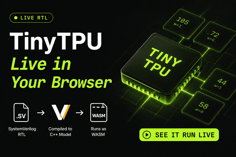
I had been using TPUs for almost a year before I realized I had absolutely no idea what was happening inside one.

I knew the math. I could write the `nn.Linear` call. I understood that matrix multiplication maps cleanly to hardware. But why it maps cleanly, what’s actually happening in the silicon when those multiplications fire was a complete mystery to me.

The standard explanation is a diagram with arrows. Weights go in here, activation's go in there, results come out the bottom. Clean. Tidy. Completely useless for actually understanding anything.

So I decided to build one. A real one. And make it run in the browser so I could watch it cycle by cycle.

That became TinyTPU.

What I Actually Wanted to Understand#

TPUs use something called a systolic array to execute matrix multiply. It’s the architecture behind why TPUs are efficient at exactly the workloads that matter for deep learning.

The word “systolic” means heartbeat. Data pulses through a grid of processing elements in lockstep with the clock, like a heartbeat. Each cell does one tiny job (multiply one number by another, add to a running total) and passes data to its neighbors. No cell talks to memory mid-computation. That’s the whole trick.

Weight-stationary dataflow, the variant TPUs use, works like this: you load matrix B into the grid as stationary weights. Each processing element holds one value permanently during the computation. Then matrix A streams in from the left edge, row by row, with a specific diagonal delay called the skew. Results accumulate downward through the grid and exit from the bottom.

Every explanatory article I found drew this as a static diagram. I needed to see it move.

The Constraint That Made It Honest#

When I built TinyGPU, the core decision was: model the concepts, not the hardware. The simulator was written in Python, the parallelism was simulated, the visualization was generated after the fact. That was fine for the learning goal.

TinyTPU had a different constraint from the start: nothing on screen is allowed to be faked.

Not “mostly real.” Not “a JavaScript approximation of what the hardware would do.” The browser had to run the actual hardware model. Every number in the visualization had to be a live signal read directly from compiled RTL.

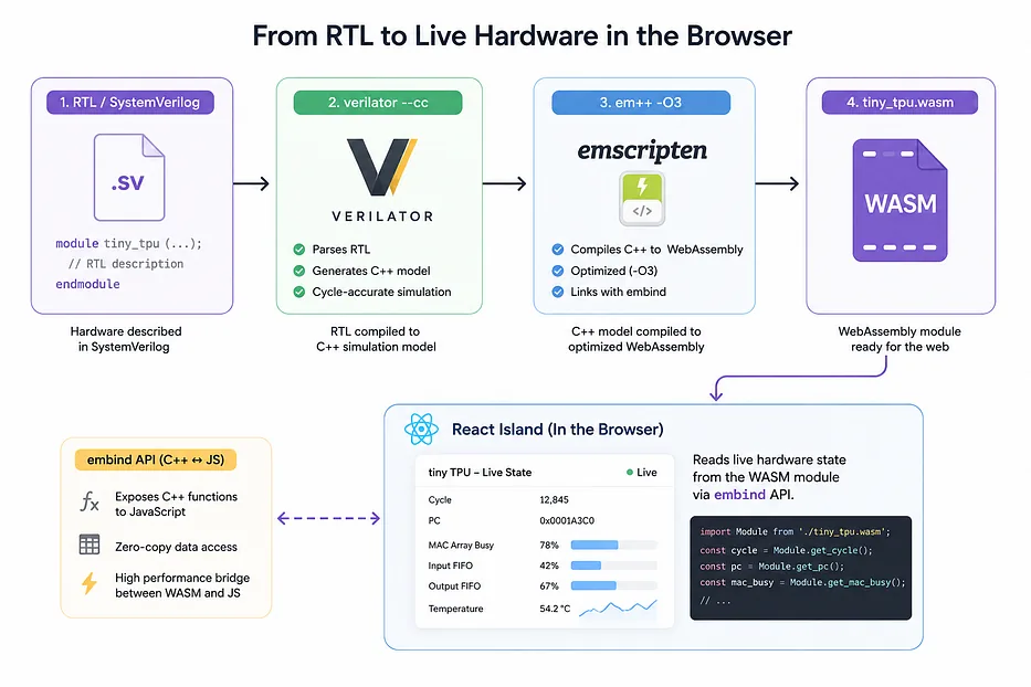
The architecture I landed on: write real synthesizable SystemVerilog, verify it with a numpy golden model, compile it to a cycle-accurate C++ simulation via Verilator, compile that to WebAssembly via Emscripten, and have the React frontend read hardware state every clock cycle through an `embind` API.

The pipeline is `.sv` → Verilator → C++ → Emscripten → `.wasm` → React island → SVG.

The Part Nobody Warned Me About: The Skew#

Here’s the thing about weight-stationary dataflow that took me an embarrassingly long time to understand from diagrams alone.

Matrix A doesn’t just stream in from the left. It streams in diagonally. Row 0 enters at cycle 0. Row 1 enters at cycle 1. Row 2 at cycle 2. And so on. This deliberate stagger called the row skew ensures that the right activation meets the right weight at the right processing element at the right clock cycle.

Without the skew, every activation would arrive at column 0 at the same time and the wrong values would multiply together. The diagonal stagger is what makes the spatial layout of the grid correspond to the temporal sequencing of the computation.

When I finally got the RTL correct and looked at the simulation waveform in gtkwave, seeing that diagonal pattern appear for the first time was genuinely satisfying. It meant the hardware was thinking the way it was supposed to think.

Three Decisions That Actually Mattered#

Decision 1: Golden model before hardware#

Before I wrote a single line of SystemVerilog, I wrote `sim/golden.py` a dead-simple numpy implementation of matrix multiply that serves as the ground truth.

Every change to the RTL gets validated against this oracle before it’s considered correct. If the hardware output bit-matches numpy for 20 random matrix pairs, the RTL is correct. If it doesn’t, it doesn’t matter how good the visualization looks, it’s a beautiful lie.

1def matmul_golden(A, B):
2return np.array(A, dtype=np.int64) @ np.array(B, dtype=np.int64)

That’s it. The simplest possible oracle. The hardware is “correct” when it matches this.

This ordering matters more than it sounds. I’ve seen hardware education projects where the author writes the visualizer first, then writes hardware that produces values that “look right.” That’s not how you learn hardware. That’s how you fool yourself.

Decision 2: The debug output bus#

Verilator can expose internal signals two ways: via a debug output bus that you explicitly wire at the top level, or via a `public_flat` flag that exposes everything.

I chose the explicit bus. Every PE’s weight, activation, and partial sum is wired to a top-level output bundle that the C++ harness reads. No reaching into internal hierarchies. No relying on compiler flags that might behave differently across Verilator versions.

1// top-level debug outputs - explicit, stable, honest
2output logic signed [ACC_W-1:0] dbg_psum [N][N],
3output logic signed [DATA_W-1:0] dbg_weight [N][N],
4output logic signed [DATA_W-1:0] dbg_act_out [N][N]

It’s more wiring. But when the visualization shows a value, you can trace exactly which RTL register it came from.

Decision 3: Never touching the WASM during SSR#

The frontend is built in Astro, which server-side renders pages at build time. WASM can’t load during SSR there’s no `window`, no browser APIs, nothing.

The fix is using `client:only=”react”` on every island that touches the simulator, and dynamically importing the WASM module inside `useEffect`. Not at the module level. Not at component top. Inside `useEffect`, after hydration, guarded by a `typeof window !== ‘undefined’` check.

I got this wrong twice before getting it right. Both times the production build was a blank white page with a cryptic error about `window is not defined`. Both times the fix was the same: move the import deeper, later, more client-side.

What Went Wrong (Several Things)#

The skew timing took the most debugging. I had the controller FSM correct and the PE wiring correct but the results were shifted one column to the right. The activation for row 0 was meeting the weight for row 1. Off by one in the per-row delay logic, which meant the diagonal stagger was starting one cycle too late.

The waveform caught it immediately once I knew what to look for: the moving diagonal was displaced by one column from where it should have been. The fix was two characters in the controller. The debugging was four hours.

The WASM bridge had its own set of problems. `verilated.cpp` not found because `VERILATOR_ROOT` was unset. The ` -Mdir` path not matching the `-I` include path. CORS blocking `.wasm` files served over `file://` (always use `python3 -m http.server` for local testing, never open directly). Each of these produced a completely different error message that didn’t point at the actual cause.

The one I didn’t expect: the whole Astro SSR/WASM problem was invisible in development and only appeared in production builds. `pnpm dev` uses a dev server that doesn’t pre-render. `pnpm build` does. You can develop locally for hours without hitting this issue and then have a broken production deploy. The fix is to run `pnpm build && pnpm preview` before calling anything done.

What It Looks Like When It Works#

The visualizer has three modes.

L1-One Cell: Isolate a single processing element. Watch the MAC equation update live: `psum_out = psum_in + weight × act_in`. See the weight load, see the activation arrive, see the partial sum update. One multiply-accumulate, made visible.

L2-The Array: The full 4×4 grid. This is the one worth watching. You see the weight loading phase (all PEs loading their stationary weights simultaneously), then the streaming phase where activations enter from the left in diagonal waves, then the drain phase as results exit from the bottom. The FSM state badge in the corner `IDLE → LOAD_WEIGHTS → STREAM → DRAIN → DONE` tracks where the hardware is in its execution.

L3-Tiling: Enter matrices larger than 4×4 and the orchestration layer splits them into 4×4 tiles, calls the real hardware repeatedly for each tile, and accumulates the results. An 8×8 matmul becomes eight passes through real RTL. The tiling itself is TypeScript that’s honest too, and documented clearly.

What This Actually Taught Me#

I can explain weight-stationary dataflow now. Not just recite the definition actually explain why you’d choose it, what tradeoff it makes (memory bandwidth for weight re-use), why it maps cleanly to matrix multiply in neural networks, and what happens at the boundaries.

I understand why tiling exists. The 4×4 array can hold 16 weights. A real `nn.Linear(1024, 1024)` has over a million weights. The hardware has to process the problem in tiles, accumulating partial results across passes. Every time a deep learning framework maps a layer to hardware, this is happening. Every time.

I also now have a reflex I didn’t have before: when something “works” in hardware simulation but produces wrong outputs, the first thing I check is timing. Not logic. Timing. The systolic array bug the off-by-one in the diagonal skew was the RTL doing exactly what I told it to do. I just told it the wrong thing by one cycle.

Building the wrong thing correctly teaches you more about the right thing than reading about the right thing ever does.

The Honest Assessment#

4 stars on GitHub at launch. That’s the number. It’s not what I hoped for.

Distribution is a separate skill from building, and I’m still learning it. The project is real verified hardware, honest signals, nothing faked. Getting people to care about that takes more than just building it correctly.

But the learning happened regardless of the star count. That’s the thing about building educational tools: the person who learns the most is always the builder.

The repo is on GitHub.

The live demo is at tiny-tpu.vercel.app.

If you want to understand what’s inside the chips running your models, this is one way to start.